Actual Effort in Cognitive Tasks

Conceptual definition of actual effort

I define actual effort as follows:

“Effort; noun; That which must be done in attempting to meet a particular task demand, or set of task demands, and which is determined by the current task demands relative to capacity to meet those demands, though cannot exceed that current capacity.”

And more specifically following Markus’¹ Set Theoretical approach as²:

“Effort (concept); $E_A(j,t,C_A,D_A,w,T_{Any})$ is the actual effort for any individual $j$ at time $t$ where $C_A(j,t,x_C)$, and $D_A(i,t,x_D)$ are the actual capacity and actual demands respectively, and $x_C$ and $x_D$ are the magnitudes of those respectively for individual $j$ at time $t$, where $w$ denotes all possible states of affairs (i.e. combinations of $j,t,C_A$, and $D_A)$, and $T_{Any}$ denotes the boundary conditions noting it as intensional to all possible types of tasks.”

And which is expressed as a derived ratio, given that capacity and demands have natural origins (capacity can be zero, as can demands, but neither can be less than zero):

$$D_A\le C_A\Rightarrow E_A=\frac{D_A}{C_A}\times 100$$

$$D_A>C_A\Rightarrow E_A=100$$

Where the ratio is expressed as a percentage (%).

Now, the $T_{Any}$ argument is important for what I am about to present. The conceptual definitions I have developed are deliberately agnostic of the type of task being performed. However, it’s not that easy to apply the definition to all kinds of tasks given that in many we haven’t got good operationalisations of $C_A$ and $D_A$. Sure, for tasks typical to my alma mater of research, resistance training, it’s pretty simple. Take a physical task such as this, in essence lifting a weight… here’s how I gave an example of the definition in play:

“In a physical task the role of differential demands and capacity are easily considered in that actual effort is determined by the task demands relative to the current capacity to meet task demands. As such, if two individuals were attempting to pick up the same specific absolute load (e.g. 80 kg) the stronger of the two would initially require less actual effort to complete this task. If they had both performed prior tasks that had resulted in a reduction in their maximal strength, then each would require a greater actual effort to complete the task than compared with when their capacity was not reduced. And further, if both continued performing repetitions of this task their maximal strength might continue to reduce insidious to continued attempts to maintain a particular absolute demand, and thus require an increasingly greater actual effort with every individual or continued attempt to meet the task demands. Correspondingly, if the absolute task demands were increased then both individuals would also require greater actual effort to complete the task. Yet for both, the continued attempted performance of the task with fixed absolute demands and insidious reduction of capacity or the increase of absolute demands, task performance would be capped by their maximum capacity at which maximum effort is required. With training though that maximum strength might be increased such that a given absolute task demand now represents relatively less and so requires less actual effort. Further, biomechanical alterations to the task might reduce the absolute demands and thus the actual effort.”

So, let’s say an individual $(j)$ did try to lift a load $(i)$ that was 80 kg. And let’s say that the maximum load they could lift was 100 kg. Well, it’s pretty simple to calculate the actual effort required:

$$D_{A(i)}=80,C_{A(j)}=100$$ $$E_{A(ji)}=\frac{D_{A(i)}}{C_{A(j)}}\times 100$$ $$80=\frac{80}{100}\times 100$$

So, the amount of actual effort required by the individual to lift the load is 80%. Nice and simple.

But what about cognitive tasks? Sure, we can conceivably apply my definition to such tasks if we assume that such tasks present demands that must be met, and that we have some capacity to meet them. In fact, we could draw similar examples as above for such tasks… again, here’s what I note:

“Similar examples could be provided for cognitive tasks. For example, if two individuals were attempting to hold a fixed number of items in their working memory, the one who has the larger working memory of the two would require less actual effort to complete this task. However, both individuals would again require greater actual effort to do so in the presence of lingering reduction in cognitive capacity from prior tasks, or from continued attempts to meet the task demands, or from increased absolute task demands (i.e., more items to be held in working memory). Again, training may also improve maximal capacity. Also, cognitive processing alterations (i.e., heuristics; Shah and Oppenheimer, 2008) might reduce task demands and thus the actual effort.”

The problem however, is actually measuring the capacity being used to perform cognitive tasks, and the demands of those tasks. It’s not as simple as with say strength or the load lifted. We have an operationalisation problem for cognitive tasks.

But, as noted, I think the trick to this problem might lie in IRT.

Item Response Theory

For those unfamiliar with IRT, I’ll provide a very brief overview of some key elements that are relevant for this post. But otherwise there are plenty of great texts out there covering its background and history, differences with Classical Test Theory, assumptions, different model types and parameters, how these are estimated, model fit etc³.

Let’s suppose that, for each person we test $j(j=1,...,J)$, and each item in a test they complete $i(i=1,...,I)$, we have a binary response $y_{ji}$ which is coded 1 for a correct answer (i.e., success), and 0 for an incorrect answer (i.e., failure). A binary IRT model aims to model $p_{ji}=P(y_{ji}=1)$; in essence the probability that a person $j$ correctly answers item $i$ which is assumed to follow a Bernoulli distribution:

$$y_{ji}\sim Bernoulli(p_{ji})$$

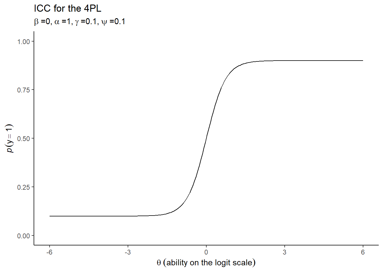
A key aspect of IRT is that, as a theory, it posits links between some construct that is a characteristic of an individual, referred to as a trait or ability, and that an individuals performance in a test of that ability are predicted or explained by that ability. However, we can’t directly observe this ability itself and instead must infer an estimation of it from the observation of performance on the test. For this reason the abilities are often referred to as latent. The relationship between the “observable” and “unobservable” is then described by a mathematical function which are models that make specific assumptions about the test data; different models imply different assumptions one is willing to make about the test data being examined given the nature of the test conducted. For example, a recently popular model due to its flexibility is the four-parameter logistic model (4PL) where $P(y_{ji}=1)$ is expressed through the equation:

$$P(y_{ji}=1)=\gamma +(1-{\gamma }_i-{\psi }_i)\frac{1}{1+exp(-({\alpha }_i{\theta }_j-{\beta }_i))}$$

In this model there are four key parameters as the name suggests, which reflect the assumptions about the test data. The ${\beta }_i$ parameter describes the item location which depending on the sign direction people prefer can refer to either the ‘difficulty’ or the ‘easiness’ of the item⁴. The ${\alpha }_i$ parameter refers to how strongly an item is related to the latent ability ${\theta }_j$ which is typically positive (i.e., that answering correctly typically implies higher ability than if answering incorrectly).The parameters ${\gamma }_i$ and ${\psi }_i$ refer to the guessing probability (i.e., that the correct answer on an item could be guessed and not due to ability), and a lapse probability respectively (i.e., that a person could make a mistake, press the wrong key etc. despite actually knowing the correct answer).

An Item Characteristic Curve (ICC) is usually used to visualise the relationship between ability and the probability of a correct response to items. So for example, a 4PL model might look something like:

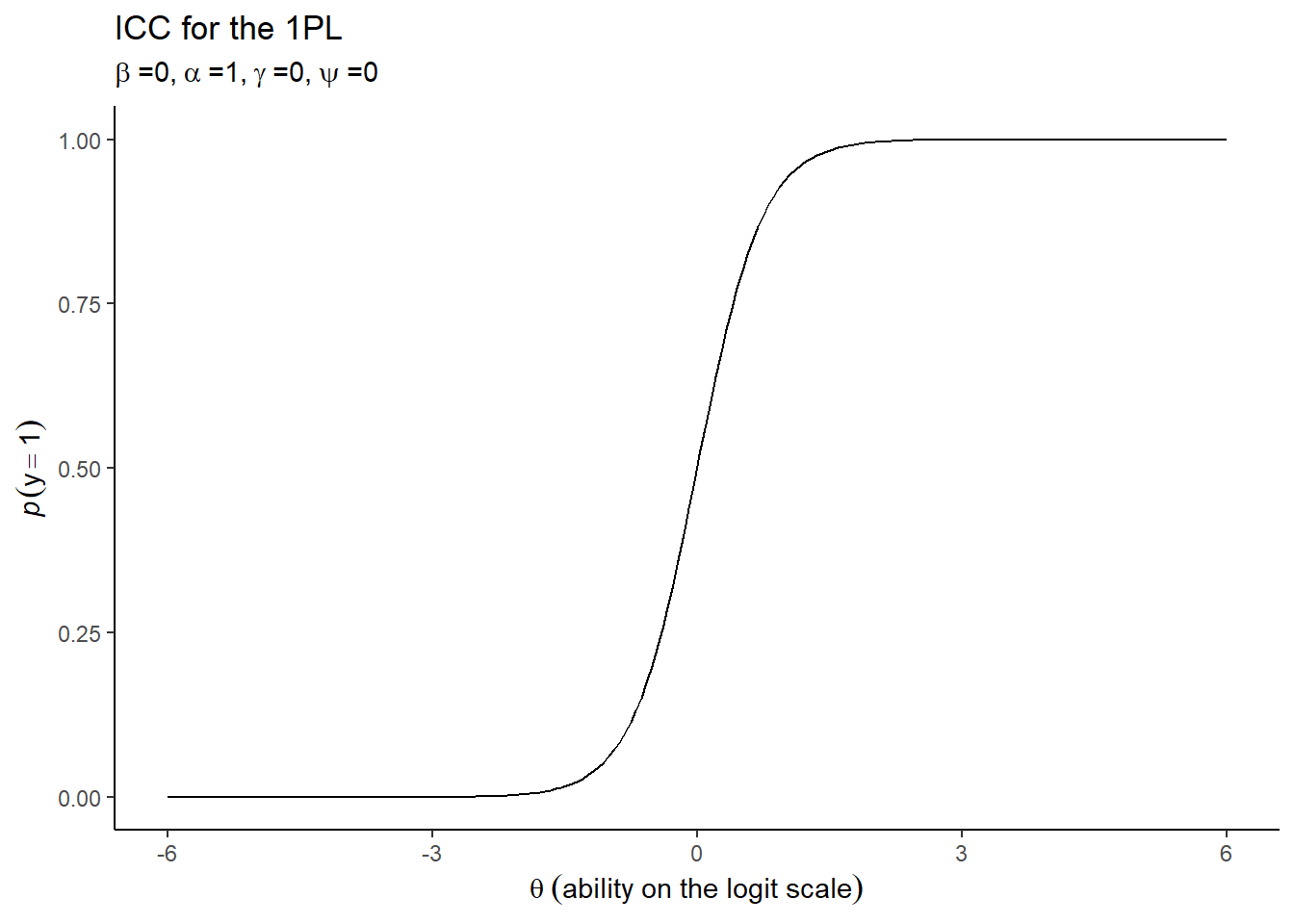
Different models make different assumptions about these parameters. For example, the simplest one-parameter logistic model (1PL or Rasch model) assumes that $\alpha =1$ and both $\gamma =0$ and $\psi =0$; that is to say, items discriminate between higher and lower abilities equally well and there is no guessing or lapses occurring. A model of that kind might look like:

In general though, the application of an IRT model allows for test data to be decomposed into an estimate of the characteristic of the individual (i.e., their ability, ${\theta }_j$). For my purpose today though, the other parameter of such models that is of primary iterest is the estimates of the test items location (i.e., their difficulty, ${\beta }_i$).

That’s about as detailed as I am going to get for the purpose of this post. The point I want to make is more conceptual… or at least, it is more about exploring whether or not we can use IRT models as a means of operationalising $C_{A(j)}$ and $D_{A(i)}$ in order to operationalise calculation of $E_{A(ji)}$ under cognitive tasks.

Ability = Capacity (${\theta }_j=C_{A(j)}$); Difficulty = Demands (${\beta }_i=D_{A(i)}$)

In essence, the argument I am putting forward here is that the two primitives $C_A$ and $D_A$ I have assumed are necessary and sufficient for the derivation of the concept $E_A$ are exactly what IRT takes as its own underlying assumed constructs; namely $\theta$ and $\beta$ respectively.

So I think that we can use IRT models in order to estimate these parameters and then use them to calculate an estimate of the $E_A$ required for each individual as they attempt each item. That is to say, we can take our function for $E_A$ above and say:

$$\beta \le \theta \Rightarrow E_{A(IRT)}=\frac{\beta }{\theta }\times 100$$

$$\beta >\theta \Rightarrow E_{A(IRT)}=100$$ Where the IRT subscript denotes that it is estimated from the IRT model.

However, those who are familiar with typical IRT models might notice a problem here for my proposed solution to operationalisation; $\beta$ and $\theta$ are typically estimated on the $logit$ scale which ranges $-\mathrm{\infty },\mathrm{\infty }$. This poses some problems for us when it comes to calculating $E_A$ given it is a ratio and the $logit$ scale does not have ratio properties.

Fortunately, the choice of which scale to place $\beta$ and $\theta$ on is rather arbitrary. Most common IRT models can undergo transformations from the $logit$ scale that both preserves the underlying probabilities for a given $\theta$ completing a given item with difficulty $\beta$. For example, the 1PL model can undergo linear transformation without altering the underlying mathematical model and we can have ${\theta }_{transf}$ and ${\beta }_{transf}$. So this gave me an idea, a toy example of sorts, to explore whether or not the derivation of effort from an IRT type model would provide a good estimate of the actual effort resultant from the demands of the task items, and the latent ability of the person performing them.

Using IRT models for lifting weights

I’m a fan of analogical abduction. I used it in developing my conceptual definition of effort in the first place. So I’m going to use the analogy of a test of the ability ‘strength’ where an individual attempts to lift different loads. In resistance training, it is pretty common to measure strength this way. We perform what is referred to as a one-repetition maximum (1RM) test. This test is the operationalisation of strength through the capacity to lift load in a given exercise task. Normally, an individual would perform a warmup, and then lift progressively heavier and heavier loads⁵ until the heaviest load they could lift only once, and no more, was identified. If we know the maximum load that an individual can lift once, then it’s a good assumption to think that this means they can also lift any load weighing less than this. If their 1RM was 100 kg and we asked them to lift 50 kg they’d almost certainly be able to. If we asked them to lift 90 kg, whilst it would be a lot more demanding to do so, they’d still almost certainly be able to do so. But if we asked them to lift 110 kg they’d almost certainly not be able to do so.

Given that the outcome of attempting to lift a given load can be considered in a binary manner (that is to say a person either can, or cannot, lift the load given their strength ability), whilst unusual to do so, we could fit an IRT model to such data. This offers an interesting toy example to play with where we could actually have a directly measurable ability (strength; $C_{A(j)}$), and also can directly measure item difficulty (loads; $D_{A(i)}$). So we can directly calculate $E_{A(j)}$ from such data. If we also fit an IRT model, transform the estimates of ${\theta }_j$ and ${\beta }_i$ back to the raw scale (i.e., kg; ${\theta }_{transf}$ and ${\beta }_{transf}$), we can then also calculate an estimate of actual effort based on the model ($E_{A(j,IRT)}$).

Let’s simulate some data⁶ and see what it looks like. We sample$n=100$ individuals from a population with a 1RM for the exercise task of $\mu =100$ kg and $sd=25$ kg, which is pretty reasonable for such a measure. We’ll say that each individual completes twenty ‘items’, which in this case means they attempt to lift twenty different loads, ranging from 10 kg to 200 kg in 10 kg intervals. Given we know their strength (i.e., $C_{A(j)}$) and the load they are trying to lift (i.e., $D_{A(j)}$) we can calculate their actual effort (i.e., $E_{A(ji)}$). Further, we can also code for their binary ‘response’ to each load; that is to say, whether they successfully lift it or not. This is determined by their strength, the same way that response to items in IRT models is assumed to be determined by the latent ability. In this case though, we know for certain whether they can or can’t lift the load given we actually know their 1RM. So we simply code 1 if 1RM is greater than or equal to the load, and 0 if 1RM is less than the load.

An example of data for an individual showing the first 10 loads looks like this⁷:

## # A tibble: 10 x 5
##    person one_RM item  actual_effort response
##    <fct>   <dbl> <fct>         <dbl>    <dbl>
##  1 p002     91.5 10             10.9        1
##  2 p002     91.5 20             21.8        1
##  3 p002     91.5 30             32.8        1
##  4 p002     91.5 40             43.7        1
##  5 p002     91.5 50             54.6        1
##  6 p002     91.5 60             65.5        1
##  7 p002     91.5 70             76.5        1
##  8 p002     91.5 80             87.4        1
##  9 p002     91.5 90             98.3        1
## 10 p002     91.5 100           100          0

Now, given the kind of test completed here (i.e., lifting different loads) it is reasonable to use the 1PL model mentioned above because there is no guessing or lapsing, nor do different items differentiate people of different abilities differently (it’s a toy example so we’re building these assumptions in). I’m going to follow an approach using Bayesian mixed effect modelling using weakly regularising priors to fit the initial 1PL model using the {brms} package which I won’t go into detail about here⁸. I’ll use Bayesian models for the following parts also with default priors to keep the approach consistent.

So we fit the 1PL model and we can plot the ICCs⁹ for each load which look like this:

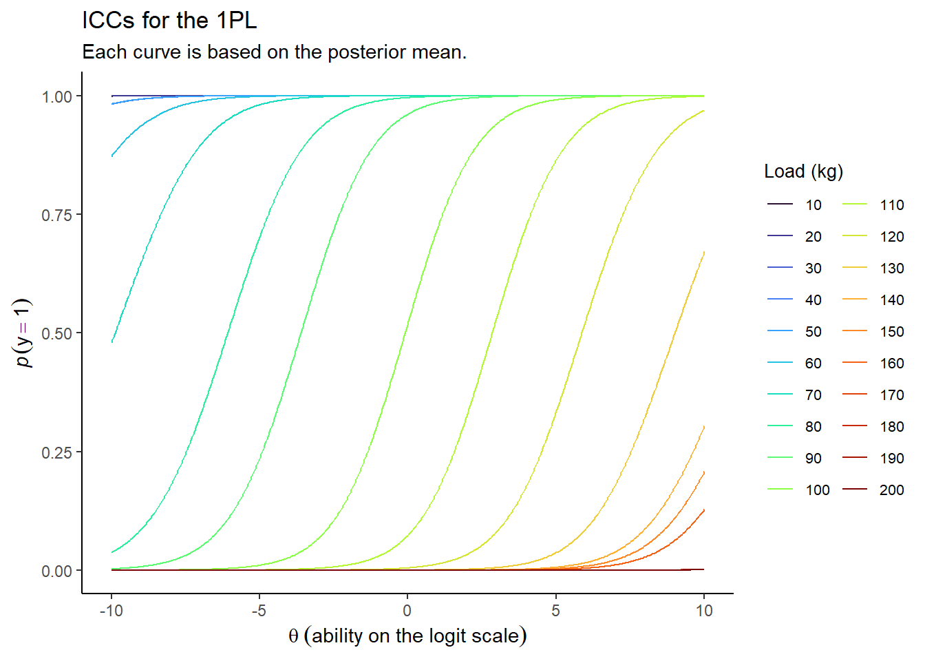
So it’s pretty clear that the model recognises that people are more likely to lift lighter loads than heavier loads, and that people with a greater strength ability are also more likely to lift a given load. We do have some loads though that are just incredibly easy such that pretty much anyone can lift them, and conversely so incredible difficult that no one can lift them.

After we fit the 1PL model we we can then extract the random effects by person and item, namely ${\theta }_j$ and ${\beta }_i$. What we want to do is examine their relationship with the ‘measured’ raw 1RM and loads respectively so we can determine the linear transformation needed to convert ${\theta }_j$ and ${\beta }_i$ back to the raw kg units ${\theta }_{j(transf)}$ and ${\beta }_{i(transf)}$.

So we fit a simple linear model to estimate 1RM from ${\theta }_j$:

lm_1RM

##  Family: gaussian 
##   Links: mu = identity; sigma = identity 
## Formula: one_RM ~ theta 
##    Data: scores_oneRM (Number of observations: 100) 
## Samples: 4 chains, each with iter = 2000; warmup = 1000; thin = 1;
##          total post-warmup samples = 4000
## 
## Population-Level Effects: 
##           Estimate Est.Error l-95% CI u-95% CI Rhat Bulk_ESS Tail_ESS
## Intercept   101.60      0.40   100.82   102.36 1.00     3512     2914
## theta         3.72      0.06     3.61     3.84 1.00     4520     3043
## 
## Family Specific Parameters: 
##       Estimate Est.Error l-95% CI u-95% CI Rhat Bulk_ESS Tail_ESS
## sigma     4.07      0.30     3.54     4.69 1.00     3747     2774
## 
## Samples were drawn using sampling(NUTS). For each parameter, Bulk_ESS
## and Tail_ESS are effective sample size measures, and Rhat is the potential
## scale reduction factor on split chains (at convergence, Rhat = 1).

And also to estimate load from ${\beta }_i$:

lm_loads

##  Family: gaussian 
##   Links: mu = identity; sigma = identity 
## Formula: load ~ beta 
##    Data: loads (Number of observations: 20) 
## Samples: 4 chains, each with iter = 2000; warmup = 1000; thin = 1;
##          total post-warmup samples = 4000
## 
## Population-Level Effects: 
##           Estimate Est.Error l-95% CI u-95% CI Rhat Bulk_ESS Tail_ESS
## Intercept   103.07      1.84    99.54   106.85 1.00     2929     2190
## beta          3.66      0.11     3.43     3.88 1.00     3147     2548
## 
## Family Specific Parameters: 
##       Estimate Est.Error l-95% CI u-95% CI Rhat Bulk_ESS Tail_ESS
## sigma     7.92      1.47     5.64    11.38 1.00     2759     2318
## 
## Samples were drawn using sampling(NUTS). For each parameter, Bulk_ESS
## and Tail_ESS are effective sample size measures, and Rhat is the potential
## scale reduction factor on split chains (at convergence, Rhat = 1).

And visually the fit looks like this:

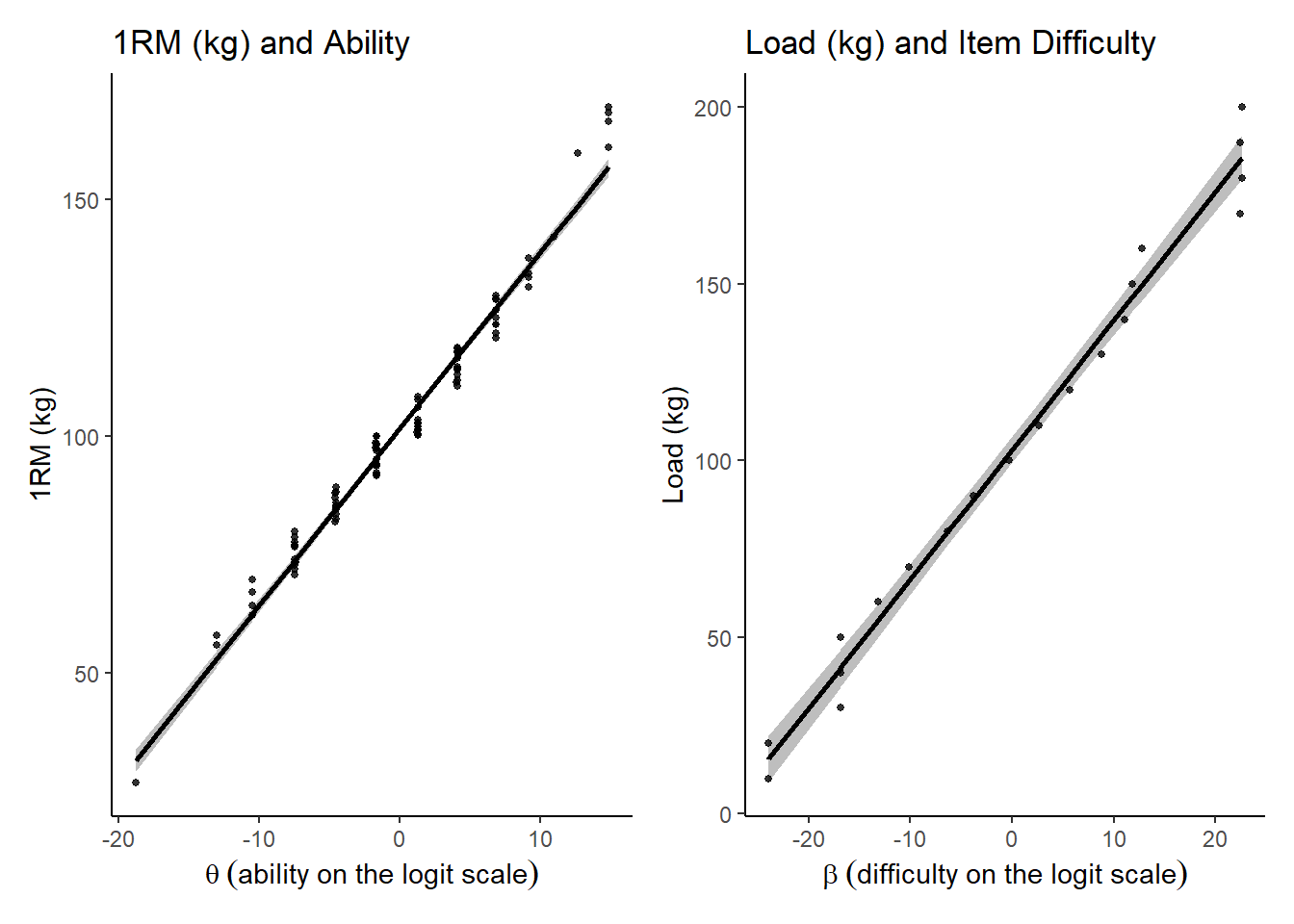
So, we can now use the intercepts and coefficients from these models to linearly transform ${\theta }_j$ and ${\beta }_i$ back to the raw kg units ${\theta }_{j(transf)}$ and ${\beta }_{i(transf)}$. Then we can use them to calculate our IRT model estimate of actual effort as:

$${\beta }_{i(transf)}\le {\theta }_{j(transf)}\Rightarrow E_{A(ji,IRT)}=\frac{{\beta }_{i(transf)}}{{\theta }_{j(transf)}}\times 100$$

$${\beta }_{i(transf)}>{\theta }_{j(transf)}\Rightarrow E_{A,(ji,IRT)}=100$$

Now we have two sets of actual effort in our dataset; we have the original actual effort calculated directly from the 1RM and loads ($E_{A(ji)}$) and also and effort calculated from our transformed estimates of ability and difficulty ($E_{A(ji,IRT)}$).

##    person   one_RM item actual_effort   theta        beta theta_to_raw
## 1    p001 103.3932   10      9.671814 1.25077 -23.9547152     106.2544
## 2    p001 103.3932   20     19.343628 1.25077 -23.9230662     106.2544
## 3    p001 103.3932   30     29.015442 1.25077 -16.8780428     106.2544
## 4    p001 103.3932   40     38.687256 1.25077 -16.8764711     106.2544
## 5    p001 103.3932   50     48.359070 1.25077 -16.8987563     106.2544
## 6    p001 103.3932   60     58.030884 1.25077 -13.2056382     106.2544
## 7    p001 103.3932   70     67.702698 1.25077 -10.1221819     106.2544
## 8    p001 103.3932   80     77.374512 1.25077  -6.3022157     106.2544
## 9    p001 103.3932   90     87.046326 1.25077  -3.8182128     106.2544
## 10   p001 103.3932  100     96.718140 1.25077  -0.2936207     106.2544
##    beta_to_raw irt_effort
## 1     15.47079   14.56013
## 2     15.58653   14.66906
## 3     41.34980   38.91583
## 4     41.35555   38.92124
## 5     41.27405   38.84454
## 6     54.77959   51.55511
## 7     66.05562   62.16740
## 8     80.02504   75.31454
## 9     89.10890   83.86370
## 10   101.99815   95.99425

Now, because we have multiple observations for each individuals we can fit a mixed effects model with random intercepts and slopes to explore how well the $E_{A(ji,IRT)}$ estimates $E_{A(ji)}$. Given the conceptualisation of effort as being a bounded construct on the 0% to 100% interval we should use a model taking that into account and so we fit an ordered beta regression model¹⁰.

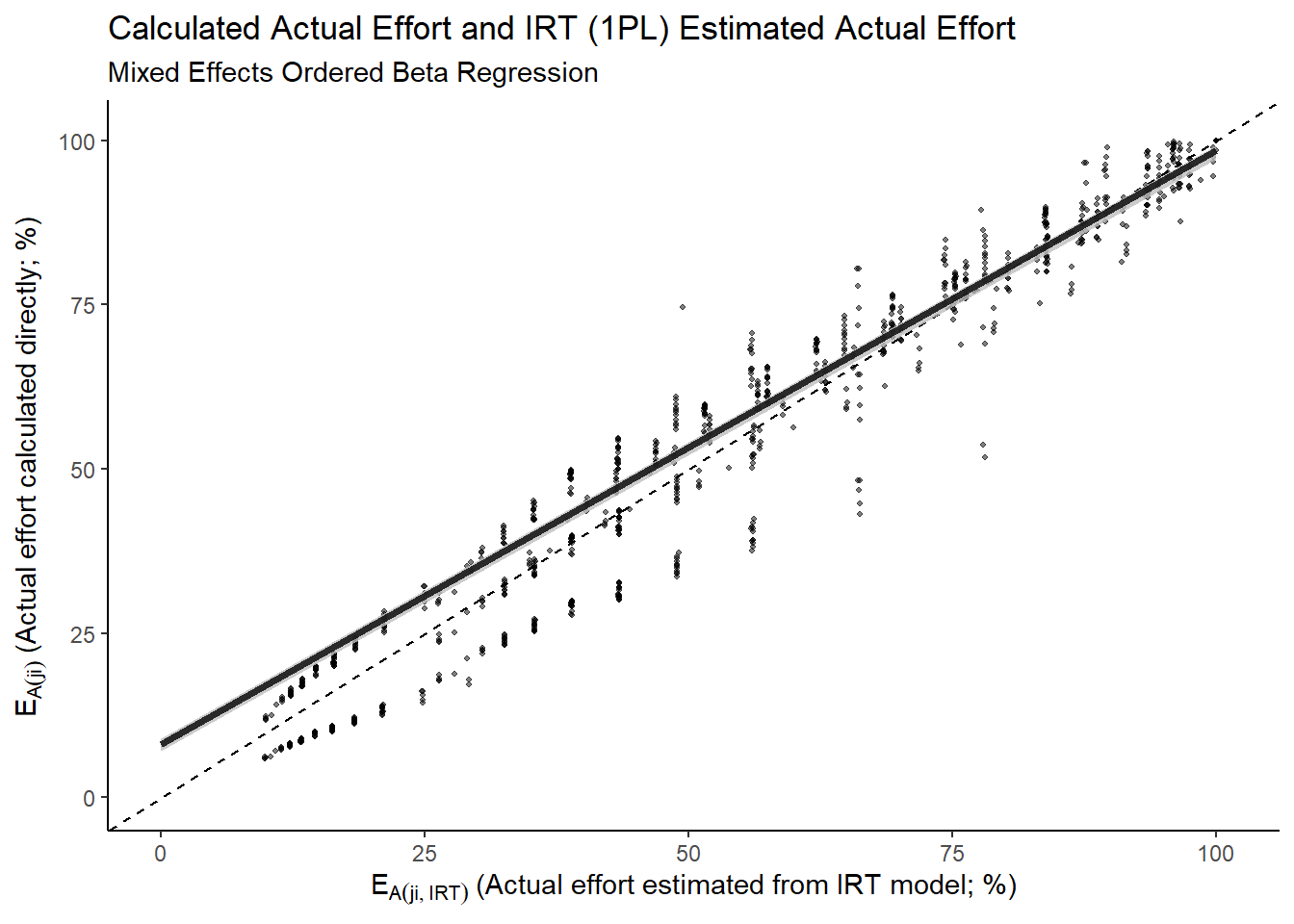
This doesn’t look too bad to be fair. In fact, while it slightly underestimates at the lower bounds, it’s pretty darn good in my opinion and leaves me feeling fairly confident in using $E_{A(ji,IRT)}$ as my operationalisation for $E_{A(ji)}$.

Summary and Conclusion

Key assumptions underlying IRT models and their parameters, ability and difficulty, map conceptually well onto the assumed primitives, capacity and demands, in my definition of effort. Given this, IRT models seem like a useful approach to operationalisation of actual effort in cognitive tasks. In fact, using the example of a test involving lifting weights where we actually know a persons underlying ability/capacity and the difficulty/demands of each item in the test, the estimates of effort that result from an IRT model are pretty reasonable estimates of the actual effort we could calculate from direct measurements.

I think this approach offers an interesting opportunity to look at actual effort in cognitive tasks. This could be particularly useful in exploring psychophysics in such tasks where we also capture self-reports of perception of effort during each item.

Further, I do not think that such models are limited to only cognitive tasks. As I have shown here, we can apply IRT models to tasks we wouldn’t typically think to. Many people have been thwarted in attempts to conceptualise effort in target based tasks such as dart throwing. However, I think that the use of IRT models could also allow the estimation of actual effort for these tasks.